Exploring graph properties
In this recipe, I show how to generate a series of graph libraries and measure
some arbitrary (honestly, not sure what they mean!) graph properties with
NetworkX. Additionally, I show how to make single-bead representations.
# Define the node counts for five different libraries. These are the same
# as those used in the tests.
node_counts = [
    {
        agx.NodeType(type_id=0, num_connections=4): 2,
        agx.NodeType(type_id=1, num_connections=2): 4,
    },
    {
        agx.NodeType(type_id=0, num_connections=4): 3,
        agx.NodeType(type_id=1, num_connections=2): 3,
        agx.NodeType(type_id=2, num_connections=2): 3,
    },
    {
        agx.NodeType(type_id=0, num_connections=3): 4,
        agx.NodeType(type_id=1, num_connections=2): 6,
    },
    {agx.NodeType(type_id=0, num_connections=4): 5},
    {
        agx.NodeType(type_id=0, num_connections=3): 2,
        agx.NodeType(type_id=1, num_connections=2): 2,
        agx.NodeType(type_id=2, num_connections=1): 2,
    },
]
Now we can iterate through and collect properties and make the layouts.
datas = {}
layouts = {}
for nc in node_counts:
    iterator = agx.TopologyIterator(node_counts=nc)
    datas[iterator.graph_type] = {}
    layouts[iterator.graph_type] = {}
    for tc in iterator.yield_graphs():
        nx_graph = tc.get_nx_graph()
        rd = nx.resistance_distance(nx_graph)
        mean_resistance_distance = np.mean(
            [j for i in rd for j in rd[i].values() if j != 0.0]
        )
        eccentricity_mean = np.mean(
            list(nx.eccentricity(nx_graph).values())
        )
        datas[iterator.graph_type][tc.idx] = {
            "eccentricity_mean": eccentricity_mean,
            "mean_resistance_distance": mean_resistance_distance,
        }
        layouts[iterator.graph_type][tc.idx]= tc.get_layout(
            layout_type="kamada",
            scale=10,
        )
In the script, I show the the plotting of these data to create:
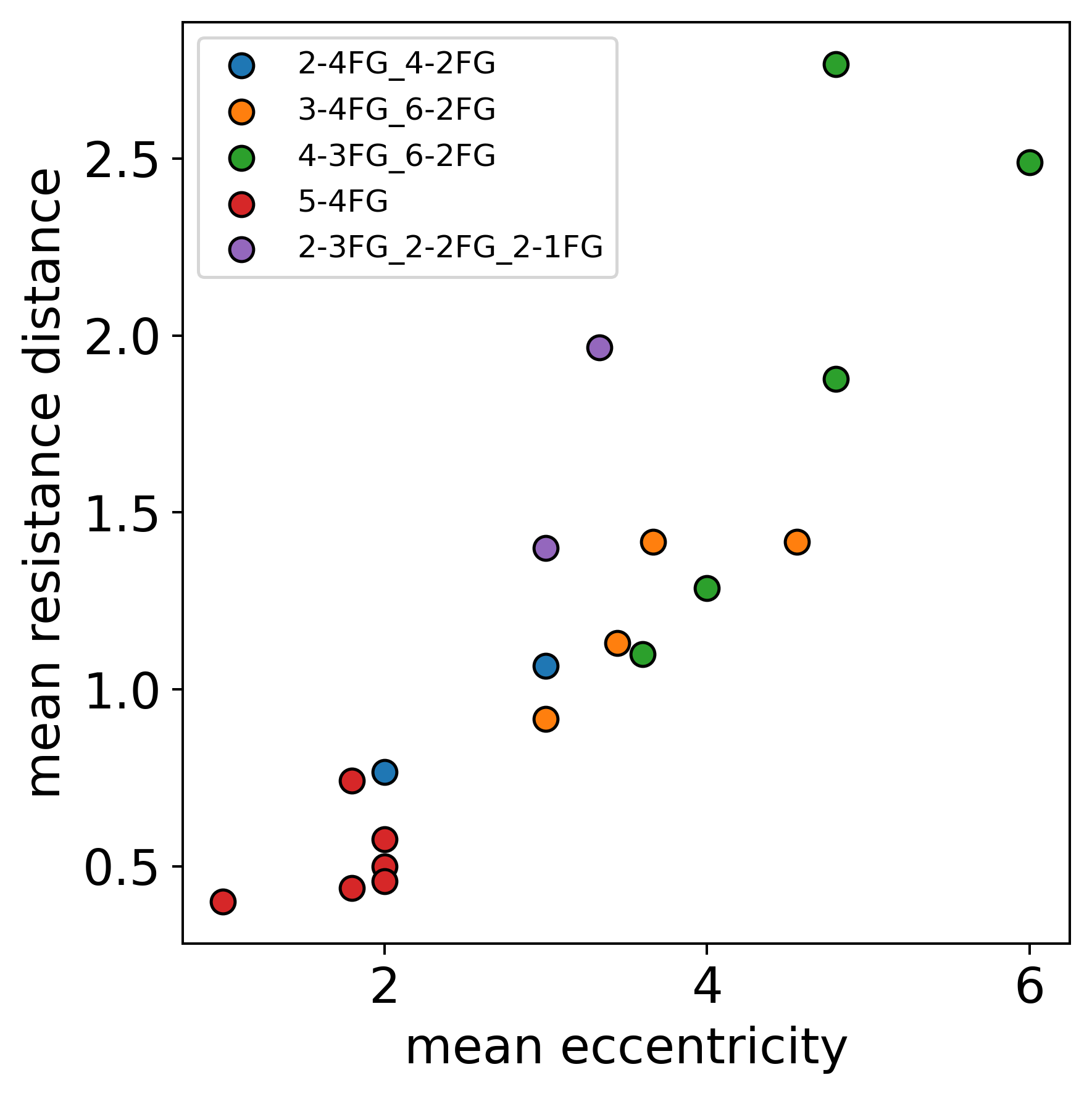
It seems there is a relationship between these two properties.
Below, I use moldoc to visualise some of these graphs, treating each node
as a carbon, like so:
iterator = agx.TopologyIterator(
    node_counts={agx.NodeType(type_id=0, num_connections=4): 5},
)
vertices_by_id = {
    i.id: i.num_connections for i in iterator.vertex_prototypes
}
for tc in iterator.yield_graphs():
    if tc.idx != 0:
        continue

    layout = tc.get_layout(layout_type="kamada", scale=5)
    moldoc_display_molecule = molecule.Molecule(
        atoms=(
            molecule.Atom(
                atomic_number=conn_color[vertices_by_id[idx]],
                position=position,
            )
            for idx, position in layout.items()
        ),
        bonds=(
            molecule.Bond(
                atom1_id=edge[0],
                atom2_id=edge[1],
                order=1,
            ) for edge in tc.vertex_map
        ),
    )
Graph of 2-4FG_4-2FG, idx = 1:
Graph of 3-4FG_6-2FG, idx = 2:
Graph of 4-3FG_6-2FG, idx = 3:
Graph of 5-4FG, idx = 2:
Graph of 2-3FG_2-2FG_2-1FG, idx = 0:
⬇️ Download Python Script